相约冬奥会

主要参考自：Hail | GWAS Tutorial^[1]本笔记旨在提供Hail功能的概述，重点是操作和查询遗传数据集的功能。我们进行了全基因组SNP关联测试，并证明了需要控制由群体分层引起的混杂。

1、安装和环境准备

#安装 Jupyter
wget https://repo.anaconda.com/miniconda/Miniconda3-latest-Linux-x86_64.sh
bash Miniconda3-latest-Linux-x86_64.sh
source miniconda3/bin/activate
conda create -n python36 python=3.6
conda activate python36
pip install hail==0.2.11
pip install jupyterlab
sudo apt-get install -y     openjdk-8-jre-headless     g++      libopenblas-base liblapack3
#配置 Jupyter
touch  venv/conf.py
#创建密码
PASSWD=$(python -c 'from notebook.auth import passwd; print(passwd("jup"))')
echo "c.NotebookApp.password = u'${PASSWD}'"
vi conf.py
c.NotebookApp.open_browser = False
c.NotebookApp.port = 8818
c.NotebookApp.password = u'sha1:｛ sha1 值｝' # ${PASSWD} 替换为实际的 sha1 值
 jupyter lab --config  ./conf.py
# 新建一个python笔记本，初始化
import hail as hl
hl.init()
# ############
using hail jar at /home/ubuntu/miniconda3/envs/python36/lib/python3.6/site-packages/hail/hail-all-spark.jar
Running on Apache Spark version 2.2.3
SparkUI available at http://10.0.8.13:4040
Welcome to
     __  __     <>__
    / /_/ /__  __/ /
   / __  / _ `/ / /
  /_/ /_/_,_/_/_/   version 0.2.11-cf54f08305d1
LOGGING: writing to /home/ubuntu/hail/hail-20220203-1927-0.2.11-cf54f08305d1.log

根据提示，看到的spark大数据的网页管理界面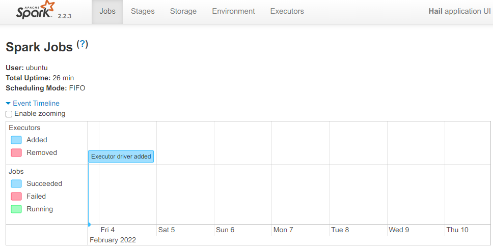在使用 Hail 之前，我们导入了一些标准的 Python 库，以便在整个笔记本中使用。

from hail.plot import show
from pprint import pprint
hl.plot.output_notebook()

这是一个类似ggplot这种包的python绘图包。

# 下载1kg数据，好像还是谷歌的网址，竟然下载成功了
# 我们使用公共1000基因组数据集的一小部分，该数据集是通过将完整VCF中的基因分型SNP缩减到约20 MB采样而创建的。我们还将集成来自单独文本文件的示例和变体元数据。
# 这些文件由Hail团队托管在公共Google存储桶中;以下命令下载该数据到本地。
hl.utils.get_1kg('data/')
# ####################
2022-02-03 19:59:22 Hail: INFO: downloading 1KG VCF ...
  Source: https://storage.googleapis.com/hail-tutorial/1kg.vcf.bgz
2022-02-03 19:59:24 Hail: INFO: importing VCF and writing to matrix table...
2022-02-03 19:59:29 Hail: INFO: Coerced sorted dataset
2022-02-03 19:59:40 Hail: INFO: wrote matrix table with 10879 rows and 284 columns in 16 partitions to data/1kg.mt
2022-02-03 19:59:40 Hail: INFO: downloading 1KG annotations ...
  Source: https://storage.googleapis.com/hail-tutorial/1kg_annotations.txt
2022-02-03 19:59:40 Hail: INFO: downloading Ensembl gene annotations ...
  Source: https://storage.googleapis.com/hail-tutorial/ensembl_gene_annotations.txt
2022-02-03 19:59:42 Hail: INFO: Done!
# 查看文件情况
!ls -lh data
# total 18M
-rw-r--r-- 1 ubuntu ubuntu 100K Feb  3 19:59 1kg_annotations.txt
drwxrwxr-x 7 ubuntu ubuntu 4.0K Feb  3 19:59 1kg.mt
-rw-r--r-- 1 ubuntu ubuntu  16M Feb  3 19:59 1kg.vcf.bgz
-rw-r--r-- 1 ubuntu ubuntu 2.5M Feb  3 19:59 ensembl_gene_annotations.txt

2、先练练手，熟悉操作

环境配置好，可以愉快地学习啦！

从 VCF 导入数据^[2]

VCF 文件中的数据自然表示为 Hail MatrixTable^[3]。通过首先导入VCF文件，然后以Hail的文件格式写入生成的 MatrixTable，这样对VCF数据的所有下游操作都将快得多。

hl.import_vcf('data/1kg.vcf.bgz').write('data/1kg.mt', overwrite=True)
# 2022-02-03 20:09:22 Hail: INFO: Coerced sorted dataset
2022-02-03 20:09:28 Hail: INFO: wrote matrix table with 10879 rows and 284 columns in 1 partition to data/1kg.mt

接下来，我们读取写入的文件，分配变量mt（matrix table）。mt = hl.read_matrix_table('data/1kg.mt')

了解我们的数据

重要的是要有简单的方法来切片、切块、查询和汇总数据集。下面演示了其中一些功能：

rows^[4] 方法可用于获取包含 MatrixTable 中所有行字段的表。

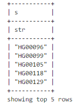
我们可以与选择^[5]一起使用以拉出5个变异。该方法采用引用表中字段名称的字符串或 Hail Expression^[6]。在这里，我们将参数留空，以仅保留行键字段和 。rows select locus alleles

mt.rows().select().show(5)
# 或者 mt.row_key.show(5)

使用该方法显示多属性。show

mt.s.show(5)

要查看前几个基因型调用，我们可以将entries^[7]与select和take一起使用。take方法将前 n 行收集到一个列表中。或者，我们可以使用show方法以表格格式将前n行打印到控制台。

尝试在下面的单元格中take更改为show。

mt.entry.take(5)
# ######
[Struct(GT=Call(alleles=[0, 0], phased=False), AD=[4, 0], DP=4, GQ=12, PL=[0, 12, 147]),
 Struct(GT=Call(alleles=[0, 0], phased=False), AD=[8, 0], DP=8, GQ=24, PL=[0, 24, 315]),
 Struct(GT=Call(alleles=[0, 0], phased=False), AD=[8, 0], DP=8, GQ=23, PL=[0, 23, 230]),
 Struct(GT=Call(alleles=[0, 0], phased=False), AD=[7, 0], DP=7, GQ=21, PL=[0, 21, 270]),
 Struct(GT=Call(alleles=[0, 0], phased=False), AD=[5, 0], DP=5, GQ=15, PL=[0, 15, 205])]

改为show看起来表格更好看：

添加列字段

Hail MatrixTable 可以具有任意数量的行字段和列字段，用于存储与每行和每列关联的数据。注释通常是任何遗传研究的关键部分。列字段用于存储有关样本表型、祖先、性别和协变量的信息。行字段可用于存储成员基因和功能影响等信息，以便在QC或分析中使用。

在本教程中，我们将演示如何获取文本文件并使用它来注释 MatrixTable 中的列。

提供的文件包含样本 ID、人口（国家）和”人口（地域）”名称、样本性别以及两种模拟表型（二分类，或离散）。

此文件可以通过import_table^[8]导入到 Hail 中。此函数生成一个 Table^[9] 对象。可以将其视为不受计算机上内存限制的Pandas或R数据帧 – 在幕后，它用Spark。

# 导入
table = (hl.import_table('data/1kg_annotations.txt', impute=True)
         .key_by('Sample'))
# #############
2022-02-07 15:09:18 Hail: INFO: Reading table to impute column types
2022-02-07 15:09:18 Hail: INFO: Finished type imputation
  Loading column 'Sample' as type 'str' (imputed)
  Loading column 'Population' as type 'str' (imputed)
  Loading column 'SuperPopulation' as type 'str' (imputed)
  Loading column 'isFemale' as type 'bool' (imputed)
  Loading column 'PurpleHair' as type 'bool' (imputed)
  Loading column 'CaffeineConsumption' as type 'int32' (imputed)

审视表格结构的一个好方法是查看其schema。

table.describe()
# #############
----------------------------------------
Global fields:
    None
----------------------------------------
Row fields:
    'Sample': str 
    'Population': str 
    'SuperPopulation': str 
    'isFemale': bool 
    'PurpleHair': bool 
    'CaffeineConsumption': int32 
----------------------------------------
Key: ['Sample']
----------------------------------------

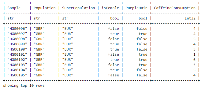
若要查看前几个值，请使用方法show:

table.show(width=100) # 100个字符？
# ########

现在，我们将使用此表将示例批注添加到数据集中，并将批注存储在 MatrixTable 的列字段中。首先，我们将打印现有的列架构（类似R语言class?）：

print(mt.col.dtype)
# struct{s: str}

我们使用annotate_cols^[10]方法将表与包含数据集的 MatrixTable 联接在一起。

mt = mt.annotate_cols(pheno = table[mt.s])
mt.col.describe()
# #############
--------------------------------------------------------
Type:
        struct {
        s: str, 
        pheno: struct {
            Population: str, 
            SuperPopulation: str, 
            isFemale: bool, 
            PurpleHair: bool, 
            CaffeineConsumption: int32
        }
    }
--------------------------------------------------------
Source:
    <hail.matrixtable.MatrixTable object at 0x7fa7f1a38278>
Index:
    ['column']
--------------------------------------------------------

查询函数和Hail表达式语言

Hail 有许多有用的查询函数，可用于收集数据集上的统计信息。这些查询函数将** Hail 表达式作为参数**。

我们将首先查看表中信息的一些统计信息。aggregate^[11]方法可用于聚合表中的行。

counter是一个聚合函数，用于计算每个唯一元素的出现次数。我们可以使用它来看人口的分布，方法是为我们要计数的字段传递Hail表达式。

pprint(table.aggregate(hl.agg.counter(table.SuperPopulation)))
# ##########
{'AFR': 1018, 'AMR': 535, 'EAS': 617, 'EUR': 669, 'SAS': 661}
2022-02-07 15:22:59 Hail: INFO: Coerced sorted dataset
# 看起来这个数据集清理不完全，好在只是警告，没报错。

stats是一个聚合函数，用于生成有关数值集合的一些有用的统计信息。我们可以用它来观察咖啡因消费表型的分布。

pprint(table.aggregate(hl.agg.stats(table.CaffeineConsumption)))
# 几个统计数字
{'max': 10.0,
 'mean': 3.983714285714278,
 'min': -1.0,
 'n': 3500,
 'stdev': 1.7021055628070707,

但是，这些指标并不能完全代表我们数据集中的样本。原因如下：

table.count()
# 3500
mt.count_cols()
# 284
mt.count_cols()
# 10879

由于数据集中的样本少于完整的千人基因组计划中的样本，因此我们需要查看数据集上的注释。我们可以使用aggregate_cols^[12]来仅获取数据集中示例的指标。

mt.aggregate_cols(hl.agg.counter(mt.pheno.SuperPopulation))
# #########少了很多样本的
{'AFR': 76, 'EAS': 72, 'AMR': 34, 'SAS': 55, 'EUR': 47}
pprint(mt.aggregate_cols(hl.agg.stats(mt.pheno.CaffeineConsumption)))
{'max': 9.0,
 'mean': 4.415492957746476,
 'min': 0.0,
 'n': 284,
 'stdev': 1.5777634274659174,
 'sum': 1253.9999999999993}

最后几个命令中演示的功能并不是什么特别新的东西：使用Pandas或R数据帧，甚至是Unix工具（如awk）来解决这些问题当然不难。但是 Hail 可以使用相同的接口和查询语言来分析要大得多的集，例如变异集。

在这里，我们计算 12 个可能的唯一 SNP 中每个 SNP 的计数（参考碱基有 4 个 * 变异碱基 3 个=12个选项）。

为此，我们需要获取每个变体的变异等位基因，然后计算每个唯一ref / alt对的出现次数。这可以通过Hail的counter功能来完成。

snp_counts = mt.aggregate_rows(hl.agg.counter(hl.Struct(ref=mt.alleles[0], alt=mt.alleles[1])))
pprint(snp_counts)
# ##########
{Struct(ref='A', alt='C'): 451,
 Struct(ref='C', alt='A'): 494,
 Struct(ref='C', alt='G'): 150,
 Struct(ref='C', alt='T'): 2418,
 Struct(ref='G', alt='A'): 2367,
 Struct(ref='A', alt='T'): 75,
 Struct(ref='T', alt='G'): 466,
 Struct(ref='G', alt='C'): 111,
 Struct(ref='G', alt='T'): 477,
 Struct(ref='A', alt='G'): 1929,
 Struct(ref='T', alt='A'): 77,
 Struct(ref='T', alt='C'): 1864}

可以使用Python的Counter类按降序列出计数。

from collections import Counter
counts = Counter(snp_counts)
counts.most_common()
# ############
[(Struct(ref='C', alt='T'), 2418),
 (Struct(ref='G', alt='A'), 2367),
 (Struct(ref='A', alt='G'), 1929),
 (Struct(ref='T', alt='C'), 1864),
 (Struct(ref='C', alt='A'), 494),
 (Struct(ref='G', alt='T'), 477),
 (Struct(ref='T', alt='G'), 466),
 (Struct(ref='A', alt='C'), 451),
 (Struct(ref='C', alt='G'), 150),
 (Struct(ref='G', alt='C'), 111),
 (Struct(ref='T', alt='A'), 77),
 (Struct(ref='A', alt='T'), 75)]

很高兴看到我们实际上可以从这个小数据集中发现一些生物学的东西：我们看到这些频率成对出现。C / T和G / A实际上是相同的突变，只是从相反的链中观察。同样，T/A 和 A/T 在相反的链上是相同的突变。C/T 和 A/T SNP 的频率之间有 30 倍的差异。为什么？

相同的Python，R和Unix工具也可以完成这项工作，但我们开始碰壁 – 最新的gnomaD版本^[13]发布了大约2.5亿个变体，并且无法在一台计算机上内存中。

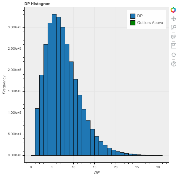
基因型呢？Hail可以查询数据集中所有基因型的集合，即使对于我们这个小数据集来说，这也越来越大。我们的 284 个样本和 10，000 个变异可产生 1000 万个独特的基因型。gnomAD数据集有大约5万亿个独特的基因型。

Hail绘制函数允许Hail字段作为参数，因此我们可以直接在此处传递 DP 字段。如果未设置范围和条柱参数，则此函数将根据字段的最小值和最大值计算范围，并使用默认的 50 个柱子。

p = hl.plot.histogram(mt.DP, range=(0,30), bins=30, title='DP Histogram', legend='DP')
show(p)

3、质控

分析师将大部分时间花在测序数据集的QC上。QC是一个迭代过程，每个项目都是不同的：QC没有”按钮”解决方案。每次Broad收集一组新的样本时，它都会发现新的批次效应。但是，通过实践开放科学并与他人讨论QC流程和决策，我们可以作为一个社区建立一套最佳实践。

QC完全基于理解数据集属性的能力。Hail 试图通过提供sample_qc^[14]函数来简化此操作，该函数生成一组有用的指标并将其存储在列字段中。

mt.col.describe()
# ##########
--------------------------------------------------------
Type:
        struct {
        s: str, 
        pheno: struct {
            Population: str, 
            SuperPopulation: str, 
            isFemale: bool, 
            PurpleHair: bool, 
            CaffeineConsumption: int32
        }
    }
--------------------------------------------------------
Source:
    <hail.matrixtable.MatrixTable object at 0x7fa7f1a38278>
Index:
    ['column']
--------------------------------------------------------
mt = hl.sample_qc(mt)
--------------------------------------------------------
Type:
        struct {
        s: str, 
        pheno: struct {
            Population: str, 
            SuperPopulation: str, 
            isFemale: bool, 
            PurpleHair: bool, 
            CaffeineConsumption: int32
        }, 
        sample_qc: struct {
            dp_stats: struct {
                mean: float64, 
                stdev: float64, 
                min: float64, 
                max: float64
            }, 
            gq_stats: struct {
                mean: float64, 
                stdev: float64, 
                min: float64, 
                max: float64
            }, 
            call_rate: float64, 
            n_called: int64, 
            n_not_called: int64, 
            n_hom_ref: int64, 
            n_het: int64, 
            n_hom_var: int64, 
            n_non_ref: int64, 
            n_singleton: int64, 
            n_snp: int64, 
            n_insertion: int64, 
            n_deletion: int64, 
            n_transition: int64, 
            n_transversion: int64, 
            n_star: int64, 
            r_ti_tv: float64, 
            r_het_hom_var: float64, 
            r_insertion_deletion: float64
        }
    }
mt.col.describe()
--------------------------------------------------------
Source:
    <hail.matrixtable.MatrixTable object at 0x7fa7f09bd240>
Index:
    ['column']
--------------------------------------------------------

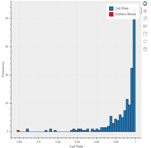
绘制 QC 指标是一个很好的起点。

p = hl.plot.histogram(mt.sample_qc.call_rate, range=(.88,1), legend='Call Rate')
show(p)

p = hl.plot.histogram(mt.sample_qc.gq_stats.mean, range=(10,70), legend='Mean Sample GQ')
show(p)

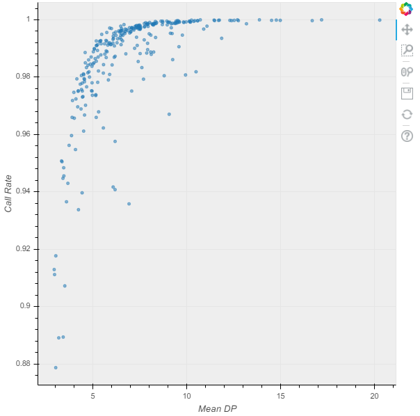
通常，这些指标是相关的。

p = hl.plot.scatter(mt.sample_qc.dp_stats.mean, mt.sample_qc.call_rate, xlabel='Mean DP', ylabel='Call Rate')
show(p)

从数据集中删除异常值通常会改善关联结果暂时没搞清楚DP，AD是啥意思，继续。我们可以进行”任意(这里应该是尝试多次的意思，歪国人喜欢搞笑)”截止，并使用它们来过滤：

mt = mt.filter_cols((mt.sample_qc.dp_stats.mean >= 4) & (mt.sample_qc.call_rate >= 0.97))
print('After filter, %d/284 samples remain.' % mt.count_cols())
# After filter, 250/284 samples remain.

接下来是基因型QC。在读数不在应该的地方过滤掉基因型是个好主意：如果我们找到一个称为纯合子参考的基因型>10%的alt reads，或者称为杂合子的基因型，没有接近1：1的ref / alt平衡，则很可能是一个错误。

在像1KG这样的低深度数据集中(PS..有点改变认知，1kG不是高深度度测序的，可是全人类的研究标准呀)，很难使用此指标检测不良基因型，因为1与10的reads比率可以很容易地用二项采样来解释。但是，在深度数据集中，10：100 的读取比率肯定会引起关注！

ab = mt.AD[1] / hl.sum(mt.AD)

filter_condition_ab = ((mt.GT.is_hom_ref() & (ab <= 0.1)) |
                        (mt.GT.is_het() & (ab >= 0.25) & (ab <= 0.75)) |
                        (mt.GT.is_hom_var() & (ab >= 0.9)))

fraction_filtered = mt.aggregate_entries(hl.agg.fraction(~filter_condition_ab))
print(f'Filtering {fraction_filtered * 100:.2f}% entries out of downstream analysis.')
mt = mt.filter_entries(filter_condition_ab)
# Filtering 3.63% entries out of downstream analysis.

变异QC 更是一样的：我们可以使用 variant_qc^[15] 函数来生成各种有用的统计数据，绘制它们并进行筛选。

mt = hl.variant_qc(mt)
mt.row.describe()
--------------------------------------------------------
Type:
        struct {
        locus: locus<GRCh37>, 
        alleles: array<str>, 
        rsid: str, 
        qual: float64, 
        filters: set<str>, 
        info: struct {
            AC: array<int32>, 
            AF: array<float64>, 
            AN: int32, 
            BaseQRankSum: float64, 
            ClippingRankSum: float64, 
            DP: int32, 
            DS: bool, 
            FS: float64, 
            HaplotypeScore: float64, 
            InbreedingCoeff: float64, 
            MLEAC: array<int32>, 
            MLEAF: array<float64>, 
            MQ: float64, 
            MQ0: int32, 
            MQRankSum: float64, 
            QD: float64, 
            ReadPosRankSum: float64, 
            set: str
        }, 
        variant_qc: struct {
            AC: array<int32>, 
            AF: array<float64>, 
            AN: int32, 
            homozygote_count: array<int32>, 
            dp_stats: struct {
                mean: float64, 
                stdev: float64, 
                min: float64, 
                max: float64
            }, 
            gq_stats: struct {
                mean: float64, 
                stdev: float64, 
                min: float64, 
                max: float64
            }, 
            n_called: int64, 
            n_not_called: int64, 
            call_rate: float32, 
            n_het: int64, 
            n_non_ref: int64, 
            het_freq_hwe: float64, 
            p_value_hwe: float64
        }
    }
--------------------------------------------------------
Source:
    <hail.matrixtable.MatrixTable object at 0x7fa7f09dd6a0>
Index:
    ['row']
--------------------------------------------------------

这些统计数据实际上看起来相当不错：我们不需要过滤这个数据集。但是，大多数数据集都需要经过深思熟虑的质量控制。filter_rows^[16]方法可以提供帮助！

4、开始GWAS！

首先，我们需要限制为以下变体：

• 常见（我们将使用 **1% **的截止值）

• 距离**哈代-温伯格均衡**^[17]不远，来发现测序错误

mt = mt.filter_rows(mt.variant_qc.AF[1] > 0.01)
mt = mt.filter_rows(mt.variant_qc.p_value_hwe > 1e-6)
print('Samples: %d  Variants: %d' % (mt.count_cols(), mt.count_rows()))
# Samples: 250  Variants: 7779

这些过滤器删除了大约15%的位点（我们从10，000多个位点开始）。这并不代表大多数测序数据集！我们已经对整整一千个基因组数据集进行了缩减采样，以包括比我们偶然预期的更常见的变体。

在 Hail 中，关联检验接受样本表型和协变量的列字段。我们已经在数据集中获得了感兴趣的表型（咖啡因消耗）：

gwas = hl.linear_regression_rows(y=mt.pheno.CaffeineConsumption,
                                 x=mt.GT.n_alt_alleles(),
                                 covariates=[1.0])
gwas.row.describe()
--------------------------------------------------------
Type:
        struct {
        locus: locus<GRCh37>, 
        alleles: array<str>, 
        n: int32, 
        sum_x: float64, 
        y_transpose_x: float64, 
        beta: float64, 
        standard_error: float64, 
        t_stat: float64, 
        p_value: float64
    }
--------------------------------------------------------
Source:
    <hail.table.Table object at 0x7fa7f0945828>
Index:
    ['row']
--------------------------------------------------------

查看上述打印输出的底部，您可以看到线性回归为 beta、标准误差、t 统计量和 p 值添加了新的行字段。

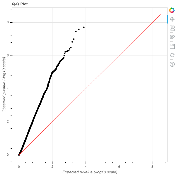
Hail使结果可视化变得容易！让我们做一个曼哈顿图^[18]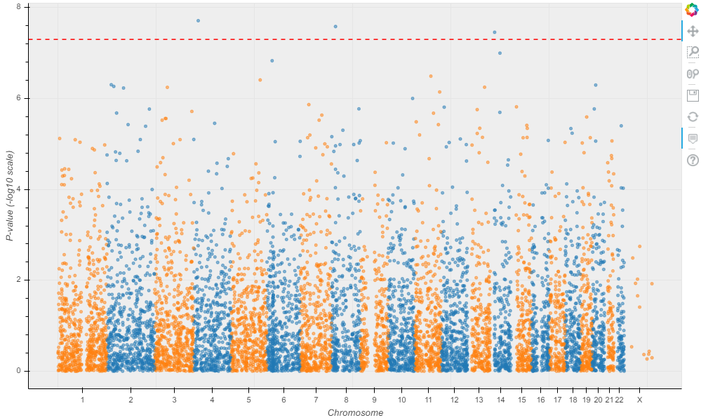：这看起来不像一个天际线。让我们检查一下我们的GWAS是否使用Q-Q（分位数-分位数）图^[19]得到了很好的控制。

p = hl.plot.qq(gwas.p_value)
show(p)

5、混淆！

观察到的 p 值会全部偏离预期。要么我们数据集中的每个SNP都与咖啡因的摄入有因果关系（不太可能），要么有一个混杂因素。

我们没有告诉你，但样本祖先实际上被用来模拟这种表型。这导致表型的**分层**^[20]分布。解决方案是在我们的回归中将祖先作为协变量包括在内。

linear_regression_rows^[21]函数还可以采用列字段作为协变量使用。我们已经用报告的祖先注释了我们的样本，但由于人为错误，对这些标签持怀疑态度是件好事。基因组没有这个问题！我们将通过使用报告的祖先，而是通过在我们的模型中包含计算的主成分来作为遗传祖先。

pca^[22] 函数将特征值生成为列表，将示例 PC 生成为表，并且还可以在询问时生成变体加载。hwe_normalized_pca^[23]函数也这样做，使用HWE归一化基因型进行PCA。

eigenvalues, pcs, _ = hl.hwe_normalized_pca(mt.GT)
# ##################
2022-02-08 09:34:10 Hail: INFO: hwe_normalized_pca: running PCA using 7771 variants.
2022-02-08 09:34:15 Hail: INFO: pca: running PCA with 10 components...
pprint(eigenvalues)
# ##########
[18.078002475659527,
 9.978057054208994,
 3.536048746504391,
 2.6583611350017096,
 1.5966283377451316,
 1.5408505989074688,
 1.5064316096906518,
 1.4747771722760974,
 1.4667919317402691,
 1.4458363475579015]
pcs.show(5, width=100)

现在我们已经为每个样本提供了主成分，我们不妨绘制它们！人类历史在遗传数据集中产生了强烈的影响。即使使用50MB的测序数据集，我们也可以恢复主要人群。

mt = mt.annotate_cols(scores = pcs[mt.s].scores)
p = hl.plot.scatter(mt.scores[0],
                    mt.scores[1],
                    label=mt.pheno.SuperPopulation,
                    title='PCA', xlabel='PC1', ylabel='PC2')
show(p)

现在，我们可以重新运行线性回归，控制样本性别和前几个主成分。我们将像以前一样使用输入变量替代等位基因的数量来执行此操作，并再次使用输入变量从PL字段导出的基因型剂量。

gwas = hl.linear_regression_rows(
    y=mt.pheno.CaffeineConsumption,
    x=mt.GT.n_alt_alleles(),
    covariates=[1.0, mt.pheno.isFemale, mt.scores[0], mt.scores[1], mt.scores[2]])
# 2022-02-08 09:49:57 Hail: INFO: linear_regression_rows: running on 250 samples for 1 response variable y,
    with input variable x, and 5 additional covariates...

我们将首先制作一个Q-Q图来评估膨胀…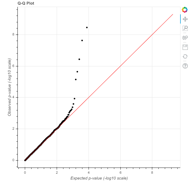这种形状表明一项控制良好（但不是特别有效）的研究。现在是曼哈顿的情节：

p = hl.plot.manhattan(gwas.p_value)
show(p)

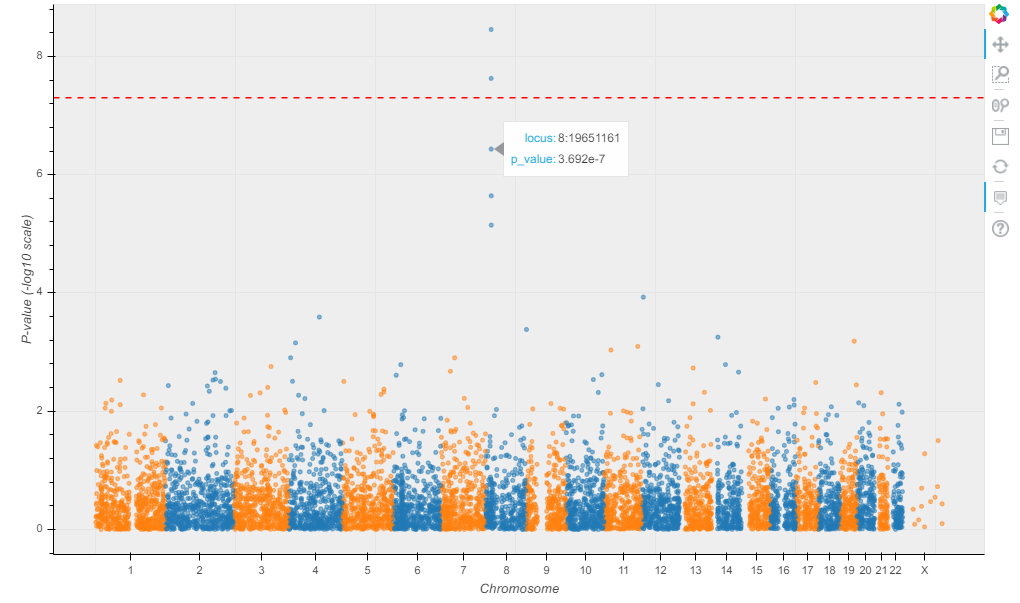我们发现了一个咖啡因的消费点！现在只需应用Hail的Nature论文功能即可发布结果。

开个玩笑，这个功能要到Hail 1.0才会登陆！

罕见变异分析

在这里，我们将演示如何使用表达式语言按行和列字段中的任何任意属性进行分组和计数。Hail 还实现了序列核心关联测检验（SKAT）。

entries = mt.entries()
results = (entries.group_by(pop = entries.pheno.SuperPopulation, chromosome = entries.locus.contig)
      .aggregate(n_het = hl.agg.count_where(entries.GT.is_het())))
results.show()

我们使用 MatrixTable.entries^[24] 方法将矩阵表转换为表（每个变体的每个样本都有一行）。在这种表示中，很容易对我们喜欢的任何字段进行聚合，这通常是罕见变体分析的第一步。

如果我们想按次要等位基因频率和头发颜色分组，并计算平均GQ，该怎么办？我们已经证明，通过几个任意统计数据很容易聚合。此特定示例可能无法提供特别有用的信息，但相同的模式可用于检测罕见变异的影响：

entries = entries.annotate(maf_bin = hl.if_else(entries.info.AF[0]<0.01, "< 1%",
                             hl.if_else(entries.info.AF[0]<0.05, "1%-5%", ">5%")))

results2 = (entries.group_by(af_bin = entries.maf_bin, purple_hair = entries.pheno.PurpleHair)
      .aggregate(mean_gq = hl.agg.stats(entries.GQ).mean,
                 mean_dp = hl.agg.stats(entries.DP).mean))
results2.show()
# module 'hail' has no attribute 'if_else'
# 有点奇怪的报错，暂未找到原因

按功能类别（同义词、错义或功能丧失）计算每个基因的杂合子基因型数量，以估计每个基因的功能约束

计算病例中每个基因的单例功能丧失突变数，并进行对照，以检测与疾病有关的基因。

结语

恭喜！您已经到了第一个教程的末尾。要了解有关 Hail 的 API 和功能的更多信息，请查看其他教程。您可以查看 Python API^[25] 以获取有关其他 Hail 函数的文档。如果您将Hail用于自己的科学，我们很乐意在Zulip聊天^[26]或论坛上收到您的来信^[27]。

作为参考，下面是合并到一个脚本中的所有教程终结点的完整流程。

table = hl.import_table('data/1kg_annotations.txt', impute=True).key_by('Sample')

mt = hl.read_matrix_table('data/1kg.mt')
mt = mt.annotate_cols(pheno = table[mt.s])
mt = hl.sample_qc(mt)
mt = mt.filter_cols((mt.sample_qc.dp_stats.mean >= 4) & (mt.sample_qc.call_rate >= 0.97))
ab = mt.AD[1] / hl.sum(mt.AD)
filter_condition_ab = ((mt.GT.is_hom_ref() & (ab <= 0.1)) |
                        (mt.GT.is_het() & (ab >= 0.25) & (ab <= 0.75)) |
                        (mt.GT.is_hom_var() & (ab >= 0.9)))
mt = mt.filter_entries(filter_condition_ab)
mt = hl.variant_qc(mt)
mt = mt.filter_rows(mt.variant_qc.AF[1] > 0.01)

eigenvalues, pcs, _ = hl.hwe_normalized_pca(mt.GT)

mt = mt.annotate_cols(scores = pcs[mt.s].scores)
gwas = hl.linear_regression_rows(
    y=mt.pheno.CaffeineConsumption,
    x=mt.GT.n_alt_alleles(),
    covariates=[1.0, mt.pheno.isFemale, mt.scores[0], mt.scores[1], mt.scores[2]])

精彩推荐

qiime2更新持续跟踪

QIIME 2 2021.2 版本发布啦
QIIME 2 2021.4发布（qiime2支持galaxy啦）
QIIME 2 2021.8到来啦
QIIME 2 2021.11发布啦

16S多段测序流程

Kraken2 Vs qiime2 16S物种注释

SMURF流程之q2-sidle（一）

SMURF流程之q2-sidle（二）– 序列重建

SMURF流程之q2-sidle（三）——数据库准备

SMURF-Science封面文章使用的16S新流程

SMURF(5R)-Science封面文章使用的16S新流程(二)

参考资料