
R和统计,R语言和统计是一对兄弟,相互难以离开呀!
这里记录下这本书里我之前不了解的内容,欢迎一起交流!向量的模式作者写了个函数来干这件事,我学习下,登上巨人的肩膀。我的理解,这个是相当于motif,计数最多的元素的意思。
mode <- function(x) {
  temp <- table(x)
  names(temp)[temp == max(temp)]
}
3.5 在R中进行多元相关分析
为避免单个变量的负面影响,以下是相关矩阵和协方差示进行多元相关分析的过程:
# 多元线性相关
data("mtcars")
# 协方差矩阵(线性相关度)
cov(mtcars[1:3])
# mpg cyl disp
# mpg 36.324103 -9.172379 -633.0972
# cyl -9.172379 3.189516 199.6603
# disp -633.097208 199.660282 15360.7998
# 相关矩阵(相关程度的大小)
cor(mtcars[1:3])
# mpg cyl disp
# mpg 1.0000000 -0.8521620 -0.8475514
# cyl -0.8521620 1.0000000 0.9020329
# disp -0.8475514 0.9020329 1.0000000
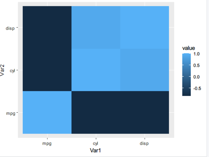
# 相关矩阵热力图
library(reshape2)
library(ggplot2)
qplot(x=Var1, y=Var2, data=melt(cor(mtcars[1:3])), fill=value, geom='tile')
3.6 进行多元回归分析
评估独立及非独立变量间的关联性
# 回归
lmfit <- lm(mtcars$mpg ~ mtcars$cyl)
lmfit
# Call:
#   lm(formula = mtcars$mpg ~ mtcars$cyl)
#
# Coefficients:
#   (Intercept)   mtcars$cyl
# 37.885       -2.876
summary(lmfit) #信息更详细?
# Call:
#   lm(formula = mtcars$mpg ~ mtcars$cyl)
#
# Residuals:
#   Min      1Q  Median      3Q     Max
# -4.9814 -2.1185  0.2217  1.0717  7.5186
#
# Coefficients:
#   Estimate Std. Error t value Pr(>|t|)
# (Intercept)  37.8846     2.0738   18.27  < 2e-16 ***
#   mtcars$cyl   -2.8758     0.3224   -8.92 6.11e-10 ***
#   ---
#   Signif. codes:  0 ‘***’ 0.001 ‘**’ 0.01 ‘*’ 0.05 ‘.’ 0.1 ‘ ’ 1
#
# Residual standard error: 3.206 on 30 degrees of freedom
# Multiple R-squared:  0.7262, Adjusted R-squared:  0.7171
# F-statistic: 79.56 on 1 and 30 DF,  p-value: 6.113e-10
# 画图
plot(mtcars$cyl,mtcars$mpg)
abline(lmfit)
稍微有点丑的图就横空出世了。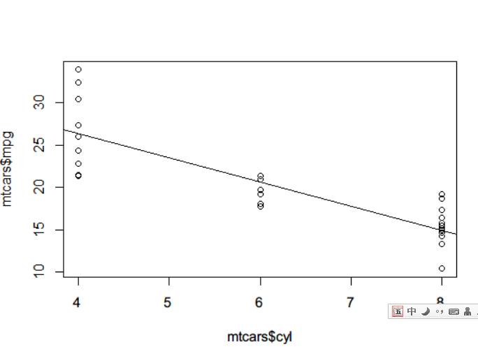 F统计可以产生一个F统计量,是模型的均方和均方误差的比值。因此,当F统计量很大时,意味着原假设被拒绝,回归模型有预测能力。
3.7 执行二项分布检验
证明假设不是偶然成立的,而是具有统计显著性。
二项分布检验
library(stats)
binom.test(x=92,n=315,p=1/6)
 Exact binomial test

data:  92 and 315
number of successes = 92, number of trials = 315, p-value = 3.458e-08
alternative hypothesis: true probability of success is not equal to 0.1666667
95 percent confidence interval:
 0.2424273 0.3456598
sample estimates:
probability of success
             0.2920635
3.8 执行t检验
boxplot(mtcars$mpg, mtcars$mpg[mtcars$am==0], ylab="mpg", name=c("overall", "automobile"))
abline(h=mean(mtcars$mpg), lwd=2, col="red")
abline(h=mean(mtcars$mpg[mtcars$am==0]), lwd=2, col="blue")
t.test(mtcars$mpg~mtcars$am)
#########################
 Welch Two Sample t-test

data:  mtcars$mpg by mtcars$am
t = -3.7671, df = 18.332, p-value = 0.001374
alternative hypothesis: true difference in means is not equal to 0
95 percent confidence interval:
 -11.280194  -3.209684
sample estimates:
mean in group 0 mean in group 1
       17.14737        24.39231

3.9 kolmogorov-smirnov检验
单样本检验用于比较样本是否符合某个已知序列(连续概率分布的相似性),双样本检验用于两个数据集累积分布方面的比较。
# 单样本
x <- rnorm(50)
ks.test(x,'pnorm')
###################
 One-sample Kolmogorov-Smirnov test

data:  x
D = 0.09625, p-value = 0.707
alternative hypothesis: two-sided
# 双样本,经验分布函数,ecdf
set.seed(3)
x<- runif(n=20, min=0,max=20)
y<- runif(n=20, min=0,max=20)
par(new=TRUE)
plot(ecdf(x), do.points=FALSE, verticals = T, xlim=c(0,20))
lines(ecdf(y), do.points=FALSE, verticals = T, lty=3)
ks.test(x,y)
##############
 Two-sample Kolmogorov-Smirnov test

data:  x and y
D = 0.3, p-value = 0.3356
alternative hypothesis: two-sided
两个p值均大于0.05,原假设成立。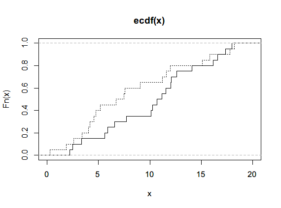
3.10 Wilcoxon秩和检验和Wilcoxon符号秩检验
非参检验,不需要假设样本服从正态分布
> wilcox.test(mtcars$mpg~mtcars$am,data=mtcars)

 Wilcoxon rank sum test with continuity correction
#############
data:  mtcars$mpg by mtcars$am
W = 42, p-value = 0.001871
alternative hypothesis: true location shift is not equal to 0

Warning message:
In wilcox.test.default(x = c(21.4, 18.7, 18.1, 14.3, 24.4, 22.8,  :
  无法精確計算带连结的p值
打结提示是因为有重复值,p值小于0.05,原假设不成立,自动和手动档汽车的mpg分布是不同的。
3.11 皮尔森卡方检验
> ftable <- table(mtcars$am, mtcars$gear)
> ftable
   ##############
     3  4  5
  0 15  4  0
  1  0  8  5
mosaicplot(ftable, main="手动和自动档前驱齿轮的马赛克图示意", color=TRUE)
 皮尔森检验,必须保证输入样本满足下面两个条件:首先,输入数据集必须都是类别数据;其次,变量必须包含两个或以上独立数据组。
R还为用户提供了其他假设检验的方法:
-
1.百分比检验prop.test: 用于测试不同样本集的百分比分布是否一致。 -
2.Z检验(UsingT包中的simple.z.test):比较样本均值与整体数据集均值以及标准偏差。 -
3.Bartlett检验(Bartlett.test):测试不同数据集的方差是否一致 -
4.Kruskal-Wallis秩和检验(kruskal.test):不确定数据集是否服从正态分布前提下,判断数据集的分布是否一致。 -
5.Shapiro-Wilk检验(shapiro.test):用于正态性检验。
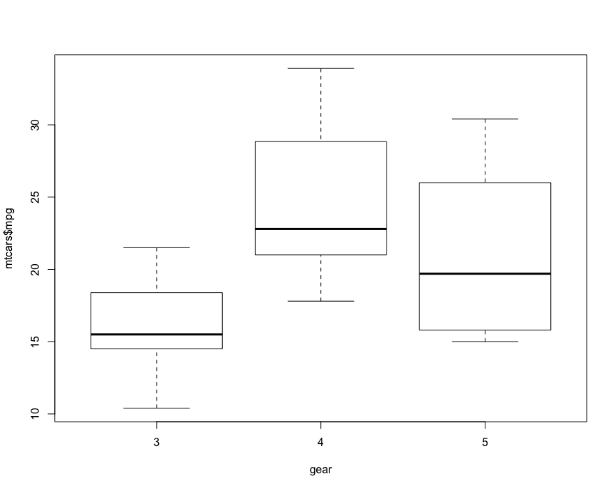
3.12 单因素方差分析
方差分析,ANOVA(Analysis of Variance),找到类别独立变量和连续非独立变量之间的关联,主要检验均值是否相同。仅包含一个类别变量作为独立变量,单因素方差分析。否则,包含两个或以上类别变量,要双因素方差分析。
# 首先,可视化
boxplot(mtcars$mpg~factor(mtcars$gear),xlab = 'gear', y='mpg')
# 然后,单因素方差分析
oneway.test(mtcars$mpg~factor(mtcars$gear))
###################该方法的优势是应用了Welch修正处理变量的不均匀性
 One-way analysis of means (not assuming equal variances)

data:  mtcars$mpg and factor(mtcars$gear)
F = 11.285, num df = 2.0000, denom df = 9.5083, p-value = 0.003085
# aov也可以,返回结果更非富
summary(aov(mtcars$mpg~as.factor(mtcars$gear)))
##################
                       Df Sum Sq Mean Sq F value   Pr(>F)
as.factor(mtcars$gear)  2  483.2  241.62    10.9 0.000295 ***
Residuals              29  642.8   22.17
---
Signif. codes:  0 ‘***’ 0.001 ‘**’ 0.01 ‘*’ 0.05 ‘.’ 0.1 ‘ ’ 1
# aov函数生成的模型也可以以表的形式输入摘要
model.tables(aov(mtcars$mpg~as.factor(mtcars$gear)))
# ############
Tables of effects

 as.factor(mtcars$gear)
         3      4     5
    -3.984  4.443 1.289
rep 15.000 12.000 5.000
# TukeyHSD事后比较检验(多重比较检验)
TukeyHSD(aov(mtcars$mpg~as.factor(mtcars$gear)))
# ##############
  Tukey multiple comparisons of means
    95% family-wise confidence level

Fit: aov(formula = mtcars$mpg ~ as.factor(mtcars$gear))

$`as.factor(mtcars$gear)`
         diff        lwr       upr     p adj
4-3  8.426667  3.9234704 12.929863 0.0002088
5-3  5.273333 -0.7309284 11.277595 0.0937176
5-4 -3.153333 -9.3423846  3.035718 0.4295874
 F-score作为组间方差和组内方差的比值,如果整体F检验显著性水平较大,可以进一步事后检验,最常用的是Scheffe、Tukey-Kramer方法和Bonferroni修正。
3.13双因素方差分析
# 同样先可视化
par(mfrow=c(1,2))
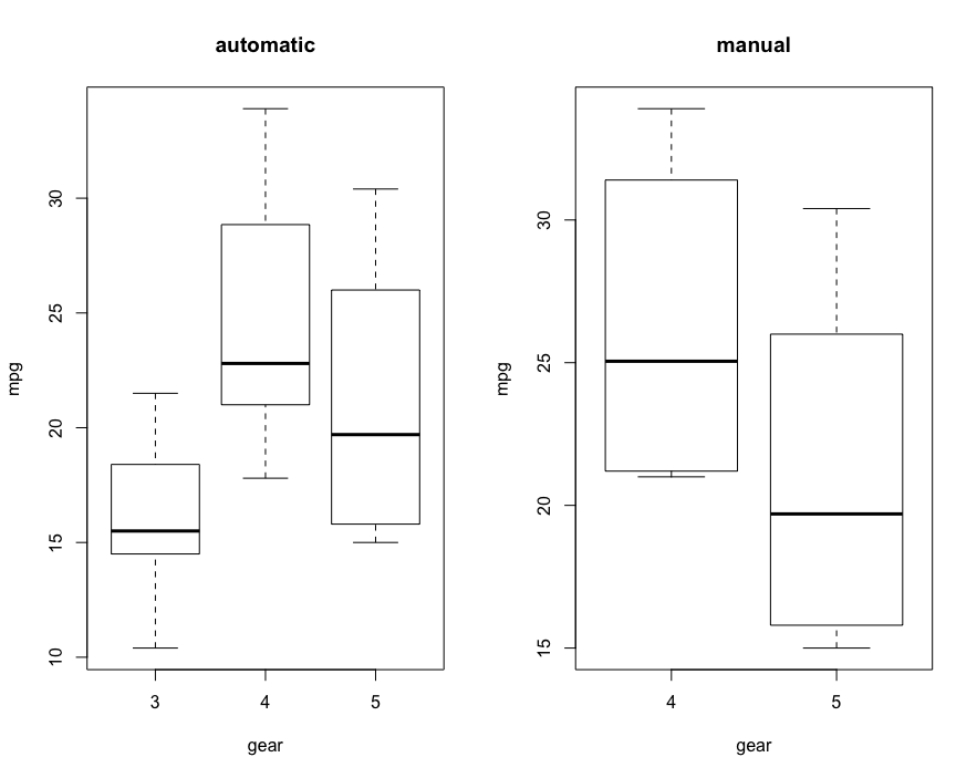
boxplot(mtcars$mpg~mtcars$gear, subset = (mtcars$am==0), xlab = 'gear', ylab = 'mpg', main='automatic')
boxplot(mtcars$mpg~mtcars$gear, subset = (mtcars$am==1), xlab = 'gear', ylab = 'mpg', main='manual')
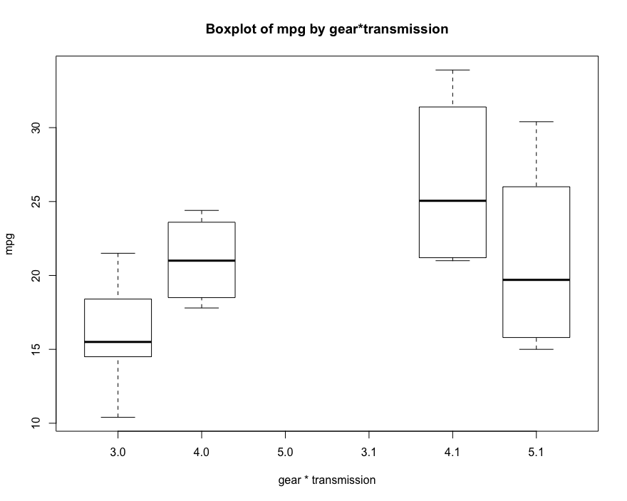
# 前驱齿轮*变速方式与mpg关联分析的盒图
boxplot(mtcars$mpg~factor(mtcars$gear)*factor(mtcars$am), xlab = 'gear * transmission', ylab = 'mpg', main='Boxplot of mpg by gear*transmission')
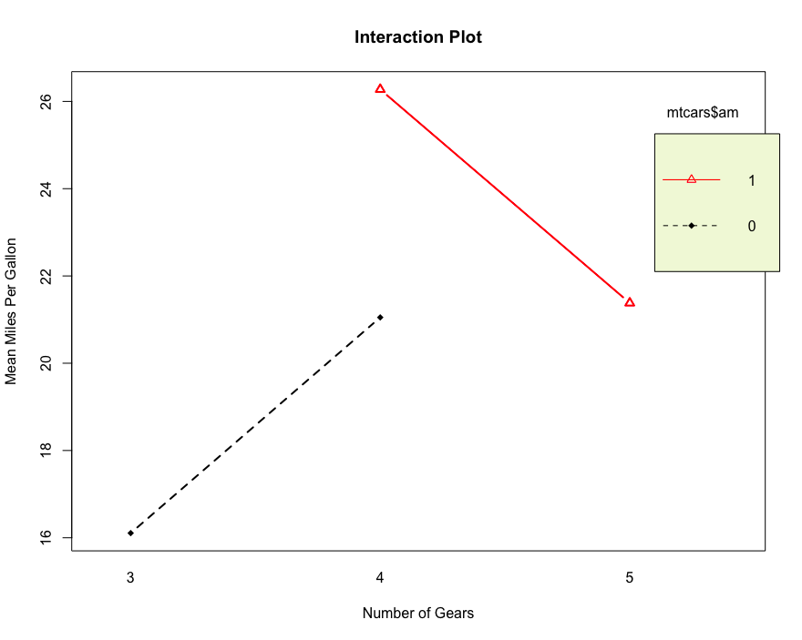
# 交互图来表达变量之间的关联
interaction.plot(mtcars$gear, mtcars$am, mtcars$mpg, type = 'b',col = c(1:3), leg.bty = 'o',leg.bg = 'beige',lwd=2, pch = c(18,24,22),
main = "Interaction Plot")
# 双因素方差分析
summary(aov(mtcars$mpg~factor(mtcars$gear)*factor(mtcars$am)))
# #################
Df Sum Sq Mean Sq F value Pr(>F)
factor(mtcars$gear) 2 483.2 241.62 11.869 0.000185 ***
factor(mtcars$am) 1 72.8 72.80 3.576 0.069001 .
Residuals 28 570.0 20.36
---
Signif. codes: 0 ‘***’ 0.001 ‘**’ 0.01 ‘*’ 0.05 ‘.’ 0.1 ‘ ’ 1
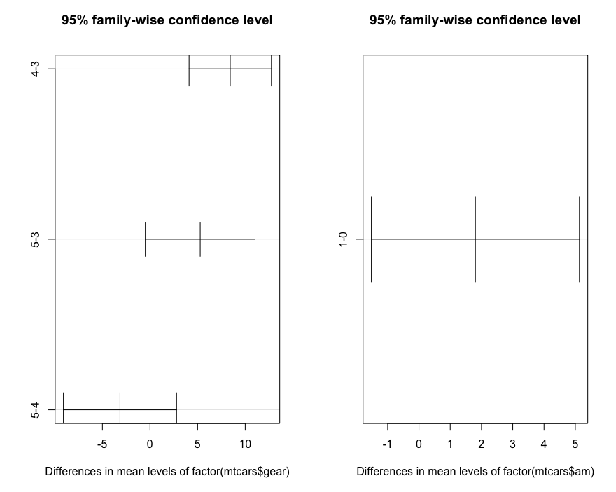
# 事后比较检验
TukeyHSD(aov(mtcars$mpg~factor(mtcars$gear)*factor(mtcars$am)))
# ###############
Tukey multiple comparisons of means
95% family-wise confidence level
Fit: aov(formula = mtcars$mpg ~ factor(mtcars$gear) * factor(mtcars$am))
$`factor(mtcars$gear)`
diff lwr upr p adj
4-3 8.426667 4.1028616 12.750472 0.0001301
5-3 5.273333 -0.4917401 11.038407 0.0779791
5-4 -3.153333 -9.0958350 2.789168 0.3999532
$`factor(mtcars$am)`
diff lwr upr p adj
1-0 1.805128 -1.521483 5.13174 0.2757926
par(mfrow=c(1,2))
plot(TukeyHSD(aov(mtcars$mpg~factor(mtcars$gear)*factor(mtcars$am))))
 扩展函数manova适用于多元变量分析,用于检验多元独立变量对多元非独立变量的影响。
欢迎微信交流
小编微信

扫描二维码
获取更多精彩
公众号

本篇文章来源于微信公众号: 微因