R、RStudio和ggplot2简介
4.1 R和RStudio简介
citation(“ggplo2”)取包引用信息,RStudio.Version()可以获取RStudio引用信息。
4.1.1 安装R、RStudio和R包
R提供一个基于命令行的统计框架,RStudio作为IDE,所有统计分析和图形可以使用它进行。
4.1.2 设置工作目录(略)
4.1.3 RStudio进行数据分析
4.1.3.1 RStudio基本特征
更加用户友好(略)
4.1.3.2 RStudio数据展示
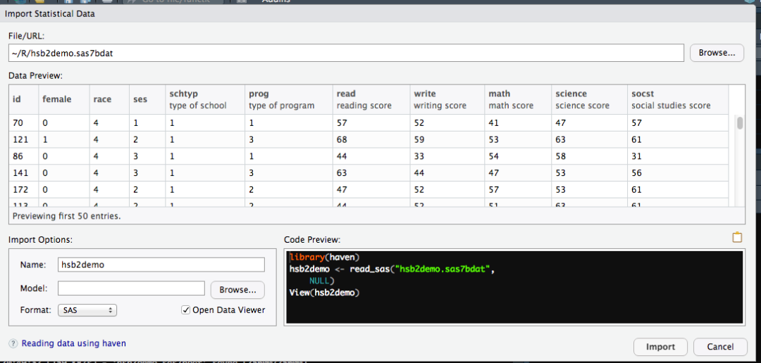
这部分是如何利用RStudio和hsbdemo(https://stats.idre.ucla.edu/wp-content/uploads/2017/06/hsb2demo.sas7bdat)数据来作一个boxplot。hsbdemo数据是SAS格式的,收集了200所高中学生不同科目的的成绩,性别中男标记为1,女0,总共200行11列。首先,下载这些数据,然后把它们放在工作目录,文件–导入数据–从SAS–选中刚下载的文件,就OK啦。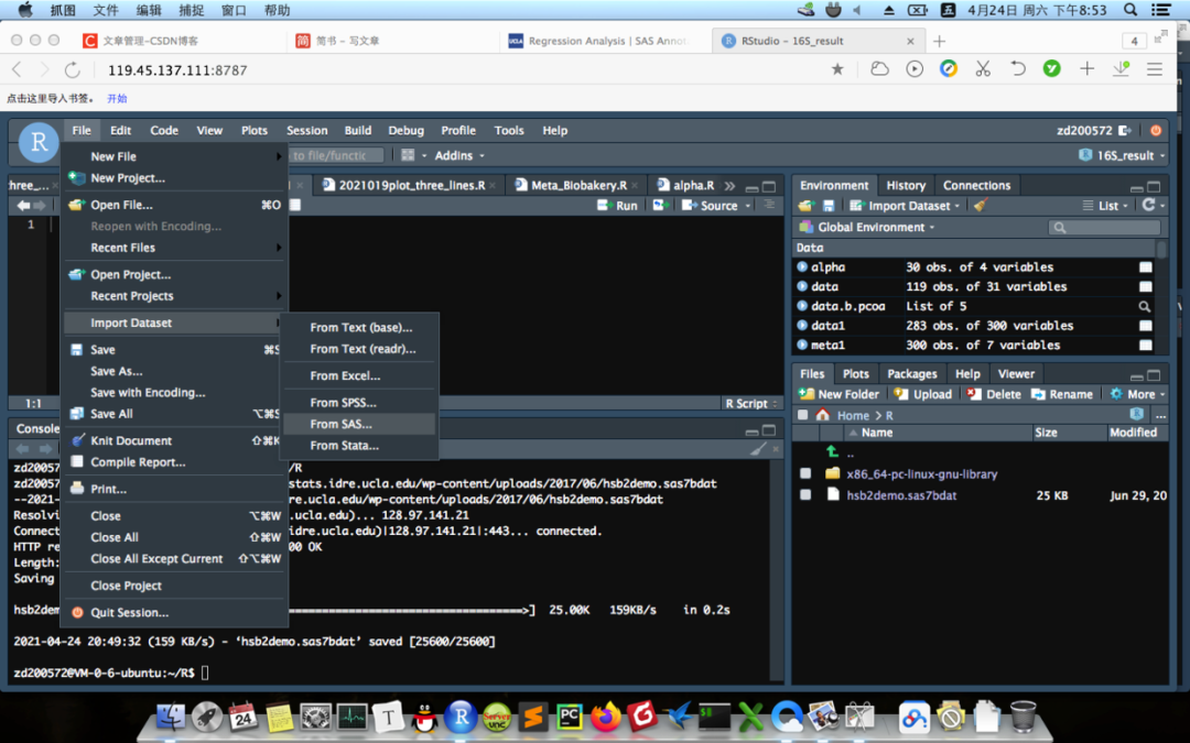
 导入后数据会自动打开,可以看到和书中描述一致的。
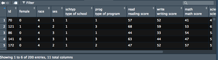 下面就是画图啦:
barplot(write~female, data = hsb2demo, main="高中学生成绩数据",xlab = "性别",ylab = "性别与写作成绩")
# Error in barplot.formula(write ~ female, data = hsb2demo, main = "高中学生成绩数据",  :
# duplicated categorical values - try another formula or subset
报错啦,重复的分类值,是啥情况呢?原来图的函数用错了,是boxplot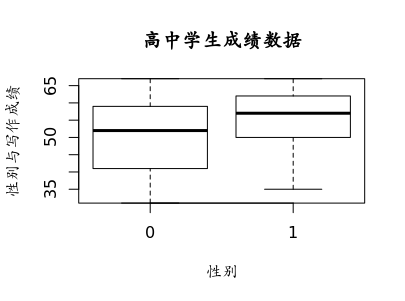 可以使用ggplot2画更高品质的图。
4.1.4 数据导入和导出
read.table(), read.csv() , read.csv2 (), read.delim() ,以及其他函数可以执行导入。stringsAsFactors=TRUE的默认选项是为了lm()/glm()这样的回归模型函数。但在基因和微生物组研究中这并不适用,因为它们多数只是标签,不用于建模。
raw<- "https://raw.githubusercontent.com/chvlyl/PLEASE/master/1_Data /Raw_Data/MetaPhlAn/PLEASE/G_Remove_unclassfied_Renormalized_M erge_Rel_MetaPhlAn_Result.xls"
tab <- read.table(raw,sep='t',header=TRUE,row.names = 1, check.names=FALSE,stringsAsFactors=FALSE)
check.names=FALSE有两个原因:1、告诉函数忽略重复变量输入(如一个样本的种级别表包含多个相同名称的种);2、另一个原因是让函数不试图去修正种的名字,来保证系统上的正确(否则,名字中的空间可能变为.)。####4.1.4.2 read.delim() read.table()提供了更多的选项,相比read.delim()。
4.1.4.3 read.csv() 和 read.csv2()
这两个函数为了不同国家中的csv文件的定义,read.csv2()是读取”;”分隔,“,”分小数的文件。read.csv()是读我们通常使用的“,”分隔,“.”分小数的文件。####4.1.4.4 gdata包 gdata包的read.xls()函数可读取excel文件,这个函数使用一个perl模块 ,需要perl安装,这是个比较古老的了,估计不是linux/mac系统不带的应该懒得装,难怪这个包这么不知名。首先这个函数把excel文件转换成csv,然后调用 read.csv()解决,这还是自己来吧!
nstall.packages("gdata")
library(gdata)
tab <- read.xls("table.xlsx",sheet=1,header=TRUE)
4.1.4.5 XLConnect包
XLConnect包可读写和操作excel文件,readWorksheetFromFile()函数会打开一个文件的一个工作表。
> install.packages ("XLConnect")
> library (XLConnect)
> tab <- readWorksheetFromFile(file = 'table.xlsx', sheet = 1, header = T, rownames = 1)
其他的包如xlsReadWrite, xlsx也可读写和操作excel文件,大同小异。
4.1.4.6 write.table() 导出数据
quote=FALSE是因为字符串一般被双引号引着,不输出引用。
> write.table(genus, file="genus_out.csv", quote=FALSE, row.names=FALSE,sep="t")
> write.table(genus, file="genus_out.txt", quote=FALSE, col.names=TRUE,sep=",")
4.1.5 基本数据操作
attributes()会输出行名,列名和class。class()可单独输出类型,dim()单独输出行列数,nrow(),ncol()分别输出行列数。
attributes(iris)
$names
[1] "Sepal.Length" "Sepal.Width"  "Petal.Length" "Petal.Width"  "Species"

$class
[1] "data.frame"

$row.names
  [1]   1   2   3   4   5   6   7   8   9  10  11  12  13  14  15  16  17  18  19  20  21  22  23  24  25  26
 [27]  27  28  29  30  31  32  33  34  35  36  37  38  39  40  41  42  43  44  45  46  47  48  49  50  51  52
 [53]  53  54  55  56  57  58  59  60  61  62  63  64  65  66  67  68  69  70  71  72  73  74  75  76  77  78
 [79]  79  80  81  82  83  84  85  86  87  88  89  90  91  92  93  94  95  96  97  98  99 100 101 102 103 104
[105] 105 106 107 108 109 110 111 112 113 114 115 116 117 118 119 120 121 122 123 124 125 126 127 128 129 130
[131] 131 132 133 134 135 136 137 138 139 140 141 142 143 144 145 146 147 148 149 150
**检查微生物数据的多0特征 **
> tab=read.csv("VdrGenusCounts.csv",row.names=1,check.names=FALSE) > #Check total zeros in the table
> sum(tab == 0)
[1] 3103
> #Check how many non-zeros in the table > sum(tab != 0)
[1] 865
一些图形函数
par()函数用来设置和查询图形参数,mar, mfcol,mfrow最常用。打印边距的大小是以文本行为单位来衡量的。标记用于指定以线数表示的页边距大小,以绘制绘图的四条边:par(mar=c(bottom, left, top, right),默认是par (mar = (c(5, 4, 4, 2) + 0.1))。mfcol,mfrow每张放几幅图,分别代表“multiple frames in rows” (mfrow) or “multiple frames in columns” (mfcol)。在同一设备上画多幅图,可以用par(mfrow), par (mfcol), par(layout), 和 par(fig), par(split.screen) ,但 par(mfrow) 最常见。par(mfrow) 两个参数,一个是图的行数,另一个是每行的列数,默认par(mfrow = c(1,1))。layout()是mfrow() 和figure()的替代,layout(matrix, widths = w; heights = h),它指示n个图的位置,w是列宽,h是行高。
ng <- layout(matrix(c(1,3,2,3),2,2, byrow=TRUE), widths=c(5,2), height=c(3,4))
layout.show(ng)
options(width=65,digits=4)# 设置输出格式

4.1.6 简单汇总统计
最常用的是summary(),其他的还有mean(), median(), min(), max()。它们经常和apply系列函数结合使用:
iris_1 <- (iris[,-5])
head(apply(iris_1,1,mean))
# [1] 2.5 2.4 2.4 2.4 2.5 2.9
apply(iris_1,2,mean)
# Sepal.Length  Sepal.Width Petal.Length  Petal.Width
#         5.8          3.1          3.8          1.2
apply(iris_1,2,mean,na.rm=T)
# Sepal.Length  Sepal.Width Petal.Length  Petal.Width
#        5.8          3.1          3.8          1.2
在微生物研究中,计算每个物种的相对丰度可以用如下的代码:tab_percent <- apply(tab, 2, function(x){x/sum(x)})再比如,过滤在做任意样本中相对丰度小于0.1%的物种:tab_p1<- tab[apply(tab_percent,1,max)>0.01]另外,过滤在半数样本中均为0的OTU:
cutoff = .5
tab_d5 <- data.frame(tab[which(apply(tab, 1, function(x){length(which (x!= 0))/length(x)}) > cutoff),])
4.1.7 其他有用的R函数
-
转置 t() -
分类和排序
sort() #升序,降序可用rev(sort())
order() #返回的是一个序号向量,升序,可以认为x[order(x)]=sort(x)
-
ifelse()R语言是向量化的,ifelse()可以遍历所有因子并避免使用循环,根据前面我们知道,循环调用函数次数超级多的话会让时间明显变长。 group <- ifelse(iris$Petal.Length < 4,1,2)高级一些的话,ifelse()还可以嵌套使用。 -
字符串分隔strsplit() strsplit("5_15_dryst","_") -
模式匹配grep()和替代gsub()正则表达式了,最常用的是 grep(模式,字符串), sub(模式,替代,字符串), gsub(模式,替代,字符串),后两者的区别是,sub()只替代第一个,gsub()替换全部。正则表达式中,R语言的通配符$,*等,如果匹配它们需要用””,如果匹配“”,得上“\”了。其他的还是和别的语言一致的。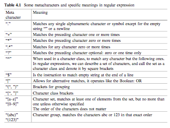
tax[1:3]
[1] Root;p__Proteobacteria;c__Betaproteobacteria;o__Neisseriales; f__Neisseriaceae;g__Neisseria
[2] Root;p__Bacteroidetes;c__Flavobacteria;o__Flavobacteriales; f__Flavobacteriaceae;g__Capnocytophaga
[3] Root;p__Actinobacteria;c__Actinobacteria;o__Actinomycetales; f__Actinomycetaceae;g__Actinomyces
# 这应该是贪婪模式,只用最后一个__?
tax_1 <- gsub(".+__", "", tax)
tax_1[1:3]
[1] "Neisseria" "Capnocytophaga" "Actinomyces"
grep()默认返回向量的元素序号,加参数value = TRUE返回值。
grep("[wd]", c("Sepal.Length", "Sepal.Width", "Petal.Length", "Petal.Width","Species"))
[1] 2 4
grep("[wd]", c("Sepal.Length", "Sepal.Width", "Petal.Length", "Petal.Width","Species"), value = TRUE)
[1] "Sepal.Width" "Petal.Width"
如果不用正则表达式,直接匹配,可以加个参数fixed =TRUE。
-
rep()和grep()这两个函数可以用来创建样本分组的信息,如:
group_1 <- data.frame(c(rep("fecal",length(grep("drySt", colnames(tab)))),rep("cecal", length(grep("CeSt", colnames(tab))))))
4.2 dplyr包简介
dplyr包提供了一系列数据操纵函数,是plyr包的第二版,专注于data frames。在以行和列转换和汇总表格数据方面,非常有用,包括选择行,过滤列、排序行,增加新列和汇总。重要的函数包括:
-
select() 和 rename() 基于名字选择列(变量) -
filter() 基于值过滤行(cases) -
arrange() 重新排序行 (cases) -
mutate() 和 transmute()创建新列, 例如, 通过已有变量,调用函数增加新的变量 -
summarise() 汇总数值 -
group_by() 分组观察值,分开和合并 -
sample_n() 和 sample_frac() 随机抽样 另外,dplyr从magrittr包引入了管道%>%,在合并几个函数时非常有用。与之前的函数嵌套从里到外调用不同,管道是从左到右依次传递,例如:
install.packages("dplyr")
library(dplyr)
head(iris)
#  Sepal.Length Sepal.Width Petal.Length Petal.Width Species
1          5.1         3.5          1.4         0.2  setosa
2          4.9         3.0          1.4         0.2  setosa
3          4.7         3.2          1.3         0.2  setosa
4          4.6         3.1          1.5         0.2  setosa
5          5.0         3.6          1.4         0.2  setosa
6          5.4         3.9          1.7         0.4  setosa
iris %>% select(Sepal.Length,Sepal.Width) %>% head
#  Sepal.Length Sepal.Width
1          5.1         3.5
2          4.9         3.0
3          4.7         3.2
4          4.6         3.1
5          5.0         3.6
6          5.4         3.9
select() 选择列
head(select(iris,Sepal.Length, Sepal.Width, Petal.Length, Petal.Width))
#  Sepal.Length Sepal.Width Petal.Length Petal.Width
1          5.1         3.5          1.4         0.2
2          4.9         3.0          1.4         0.2
3          4.7         3.2          1.3         0.2
4          4.6         3.1          1.5         0.2
5          5.0         3.6          1.4         0.2
6          5.4         3.9          1.7         0.4
head(select(iris,Sepal.Length:Petal.Width)) #同样效果
# 排除某列
head(select(iris,-Species)) #和上面同样效果
# 排除多列
head(select(iris,-(Petal.Width:Species)))
#  Sepal.Length Sepal.Width Petal.Length
1          5.1         3.5          1.4
2          4.9         3.0          1.4
3          4.7         3.2          1.3
4          4.6         3.1          1.5
5          5.0         3.6          1.4
6          5.4         3.9          1.7
还有另外的函数,基于特定标准选择列,使用select(),例如:starts_with()#起始字符, ends_with()#结束字符, matches()#正则表达式, contains()#匹配一个字符常量, 和 one_of (),基本看意思能够理解功能了。
# 匹配开头是S的列
head(select(iris,starts_with("S")))
#  Sepal.Length Sepal.Width Species
1          5.1         3.5  setosa
2          4.9         3.0  setosa
3          4.7         3.2  setosa
4          4.6         3.1  setosa
5          5.0         3.6  setosa
6          5.4         3.9  setosa
filter() 选择行
# 选择Sepal.Length>=6的行
filter(iris,Sepal.Length>=6)
 #  Sepal.Length Sepal.Width Petal.Length Petal.Width    Species
1           7.0         3.2          4.7         1.4 versicolor
2           6.4         3.2          4.5         1.5 versicolor
3           6.9         3.1          4.9         1.5 versicolor
# 选择Sepal.Length>=6 Sepal.Width>=3的行
filter(iris,Sepal.Length>=6,Sepal.Width>=3)
#   Sepal.Length Sepal.Width Petal.Length Petal.Width    Species
1           7.0         3.2          4.7         1.4 versicolor
2           6.4         3.2          4.5         1.5 versicolor
3           6.9         3.1          4.9         1.5 versicolor
arrange() 重新排序行
和flter()类似,但是只是重新排序
head(arrange(iris,Sepal.Length,Sepal.Width))
#  Sepal.Length Sepal.Width Petal.Length Petal.Width Species
1          4.3         3.0          1.1         0.1  setosa
2          4.4         2.9          1.4         0.2  setosa
3          4.4         3.0          1.3         0.2  setosa
4          4.4         3.2          1.3         0.2  setosa
5          4.5         2.3          1.3         0.3  setosa
6          4.6         3.1          1.5         0.2  setosa
默认升序,desc()降序
head(arrange(iris,desc(Sepal.Length,Sepal.Width)))
 Sepal.Length Sepal.Width Petal.Length Petal.Width   Species
1          7.9         3.8          6.4         2.0 virginica
2          7.7         3.8          6.7         2.2 virginica
3          7.7         2.6          6.9         2.3 virginica
4          7.7         2.8          6.7         2.0 virginica
5          7.7         3.0          6.1         2.3 virginica
6          7.6         3.0          6.6         2.1 virginica
# 使用管道,把前面几个函数一起用,至少比嵌套调用整洁好看和理解些吧
iris %>% select(-Species) %>% arrange(desc(Sepal.Length,Sepal.Width)) %>% head
#  Sepal.Length Sepal.Width Petal.Length Petal.Width
1          7.9         3.8          6.4         2.0
2          7.7         3.8          6.7         2.2
3          7.7         2.6          6.9         2.3
4          7.7         2.8          6.7         2.0
5          7.7         3.0          6.1         2.3
6          7.6         3.0          6.6         2.1
创建新列mutate()
head(mutate(iris,average_sepal_length=sum(Sepal.Length)/n()))
#  Sepal.Length Sepal.Width Petal.Length Petal.Width Species
1          5.1         3.5          1.4         0.2  setosa
2          4.9         3.0          1.4         0.2  setosa
3          4.7         3.2          1.3         0.2  setosa
4          4.6         3.1          1.5         0.2  setosa
5          5.0         3.6          1.4         0.2  setosa
6          5.4         3.9          1.7         0.4  setosa
  average_sepal_length
1             5.843333
2             5.843333
3             5.843333
4             5.843333
5             5.843333
6             5.843333
# 只保留新列
head(transmute(iris,average_sepal_length=sum(Sepal.Length)/n()))
  average_sepal_length
1             5.843333
2             5.843333
3             5.843333
4             5.843333
5             5.843333
6             5.843333
summarise() 汇总数值
使用这些函数mean(), sd(), min(), max(), median(), sum(), n(), first(), last() and n_distinct()。
# 把数据框变成一个单行
summarise(iris, avg_L = mean(Sepal.Width, na.rm = TRUE))
#     avg_L
1 3.057333
summarise(iris, avg_W = mean(Sepal.Width),avg_L= mean(Sepal.Length))
#     avg_W    avg_L
1 3.057333 5.843333
group_by() 分组观察值,分开和合并
iris %>% group_by(Species) %>% summarise( avg_W = mean(Sepal.Width),avg_L= mean(Sepal.Length))
`summarise()` ungrouping output (override with `.groups` argument)
# A tibble: 3 x 3 这是tibble是特殊的data.frame
  Species    avg_W avg_L
  <fct>      <dbl> <dbl>
1 setosa      3.43  5.01
2 versicolor  2.77  5.94
3 virginica   2.97  6.59
sample_n() 和 sample_frac() 随机抽样
sample_n(iris,6) #按个数抽样
#  Sepal.Length Sepal.Width Petal.Length Petal.Width    Species
1          6.7         3.1          4.7         1.5 versicolor
2          5.2         2.7          3.9         1.4 versicolor
3          4.4         2.9          1.4         0.2     setosa
4          5.9         3.2          4.8         1.8 versicolor
5          6.0         2.2          4.0         1.0 versicolor
6          5.9         3.0          4.2         1.5 versicolor
sample_frac(iris, 0.02) #按比例
#  Sepal.Length Sepal.Width Petal.Length Petal.Width    Species
1          5.7         2.5          5.0         2.0  virginica
2          5.3         3.7          1.5         0.2     setosa
3          5.1         2.5          3.0         1.1 versicolor
sample_frac(iris, 0.02,replace = TRUE) #bootstrap重采样
#  Sepal.Length Sepal.Width Petal.Length Petal.Width   Species
1          6.3         3.3          6.0         2.5 virginica
2          6.9         3.2          5.7         2.3 virginica
3          5.0         3.2          1.2         0.2    setosa
扫描二维码
获取更多精彩
公众号

本篇文章来源于微信公众号: 微因